.Buildings.DHC.Loads.BaseClasses.FlowDistribution

Information

This model represents a two-pipe hydraulic distribution system serving multiple terminal units. It is primarily intended to be used in conjunction with models that extend Buildings.DHC.Loads.BaseClasses.PartialTerminalUnit. The typical model structure for a whole building connected to an energy transfer station (or a dedicated plant) is illustrated in the schematics in the info section of Buildings.DHC.Loads.BaseClasses.PartialBuilding.

The pipe network modeling is decoupled between a main distribution loop and several terminal branch circuits:

• The mass flow rate in each branch circuit is equal to the mass flow rate demand yielded by the terminal unit model, constrained by the condition that the sum of all demands is lower or equal to the flow rate in the main loop. Additionally if the total flow rate demand exceeds the nominal mass flow rate the model generates an error.
• The inlet temperature in each branch circuit is equal to the supply temperature in the main loop. The outlet temperature in the main loop results from transferring the enthalpy flow rate of each individual fluid stream to the main fluid stream.
• The pressure drop in the main distribution loop corresponds to the pressure drop over the whole distribution system (the pump head). It is governed by an equation representing the control logic of the distribution pump.

Optionally:

• A distribution pump can be modeled with a prescribed flow rate corresponding to the total flow rate demand.
• A mixing valve can be modeled (together with a distribution pump) with a control loop tracking the supply temperature. Note that the nominal pressure drop of the valve is not an exposed parameter: it is set by default to 10% of the nominal total pressure drop.

Implementation

The modeling approach aims to minimize the number of algebraic equations by avoiding an explicit modeling of the terminal actuators and the whole flow network. In addition, the assumption allowFlowReversal=false is used systematically together with boundary conditions which actually ensure that no reverse flow conditions are encountered in simulation. This allows directly accessing the inlet enthalpy value of a component from the fluid port port_a with the built-in function inStream. This approach is preferred to the use of two-port sensors which introduce a state to ensure a smooth transition at flow reversal. All connected components must meet the same requirements. The impact on the computational performance is illustrated below.

Pump head computation

The pump head is computed as follows (see also Buildings.DHC.Loads.BaseClasses.Validation.FlowDistributionPumpControl for a comparison with an explicit modeling of the piping network).

• In case of a constant pump head,

  dpPum = dp_nominal.

• In case of a constant flow rate (three-way valves) the network flow characteristics is considered independent from the actuator positions. Hence,

  dpPum = dp_nominal.

• In case of a linear head,

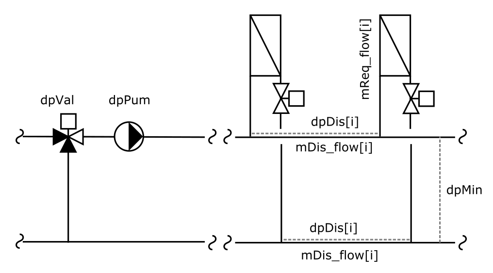
  dpPum = dpMin + (dp_nominal - dpMin) * m_flow / m_flow_nominal.

• In case of a constant speed, the pump head is computed based on the pump pressure curve and the total required mass flow rate.
• In case of a constant pressure difference at a given location, the pump head is computed according to the schematics hereunder, under the assumption of a two-pipe distribution system,

  dpPum = dpMin + dpVal + 2 * Σ_i dpDis[i],

  where

  • dpMin is the differential pressure set point.
  • dpVal is the pressure drop across the optional mixing valve. It is considered independent from the valve position, i.e., dpVal = dpVal_nominal,
  • dpDis[i] is the pressure drop in the supply pipe segment directly upstream the i^th connection,

    dpDis[i] = 1 / K[i]² * mDis_flow[i] ²,

    where mDis_flow[i] = Σ_{i to nUni} mReq_flow[i] is the mass flow rate in the same pipe segment, and K[i] = (Σ_{i to nUni} mUni_flow_nominal[i]) / dpDis_nominal[i]^0.5 is the corresponding flow coefficient (constant).

• The pressure drop in the corresponding pipe segment of the return line is considered equal, hence the factor of 2 in the above equation.

  The default value for dpDis_nominal corresponds to a configuration where the differential pressure sensor is located before the most remote connected unit, 20% of the nominal pressure drop in the distribution network occurs between the pump and the first connected unit (supply and return), the remaining pressure drop is evenly distributed over each pipe segment between the other connected units. The user can override these default values with the requirement that the nominal pressure drop of each pipe segment downstream of the differential pressure sensor must be set to zero.

Energy and mass dynamics

The energy dynamics and the time constant used in the ideal heater and cooler model are exposed as advanced parameters. They are used to represent the typical dynamics over the whole piping network, from supply to return. The mass dynamics are by default identical to the energy dynamics.

Simplifying assumptions are used otherwise, namely

• the pump is modeled in steady-state, and
• the valve and the flow splitter are modeled with fixed initial conditions. This is because the temperature of the fluid leaving the valve is used as a control input signal. If a steady-state model is used, that temperature is computed by assuming ideal mixing at the inner fluid ports of the valve. In case of zero flow rate, the temperature value results from regularizing the corresponding equation that is not well defined in that domain. That triggers non-physical temperature variations which themselves lead to control transients when the flow rate gets reestablished. Those effects turn out to be detrimental to computational performance.

Computational performance

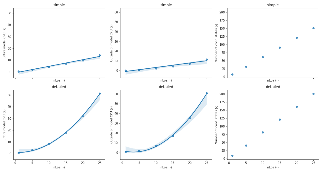
The figure below compares the computational performance of this model (labelled simple, see model Buildings.DHC.Loads.BaseClasses.Validation.BenchmarkFlowDistribution1) with an explicit modeling of the distribution network and the terminal unit actuators (labelled detailed, see model Buildings.DHC.Loads.BaseClasses.Validation.BenchmarkFlowDistribution2). The models are simulated with the solver CVODE from Sundials. The impact of a varying number of connected loads, nLoa, is assessed on

1. the total time for all model evaluations,
2. the total time spent between model evaluations, and
3. the number of continuous state variables.

A linear, resp. quadratic, regression line and the corresponding confidence interval are also plotted for the model labelled simple, resp. detailed.

Revisions

• August 30, 2022, by Hongxiang Fu:
  Swapped the pump models for preconfigured versions and removed the pump curve record per. This is for #3099.
• December 12, 2021, by Michael Wetter:
  Added parameter assignment for pumFlo.per.V_flow and pumFlo.per.pressure. This avoids in OPTIMICA a compiler error "Could not evaluate binding expression for structural parameter 'disFloHea.pumFlo.eff.per.pressure.V_flow'".
• February 21, 2020, by Antoine Gautier:
  First implementation.